Introduction

Deep generative models have shown an incredible results in producing highly realistic pieces of content of various kind, such as images, texts, and music. The three most popular generative model approaches are Generative Adversarial Networks (GANs), autoregressive models, and Variational Autoencoders (VAEs). However, this blogpost will only be focusing on VAEs.

What are Variational Autoencoders?

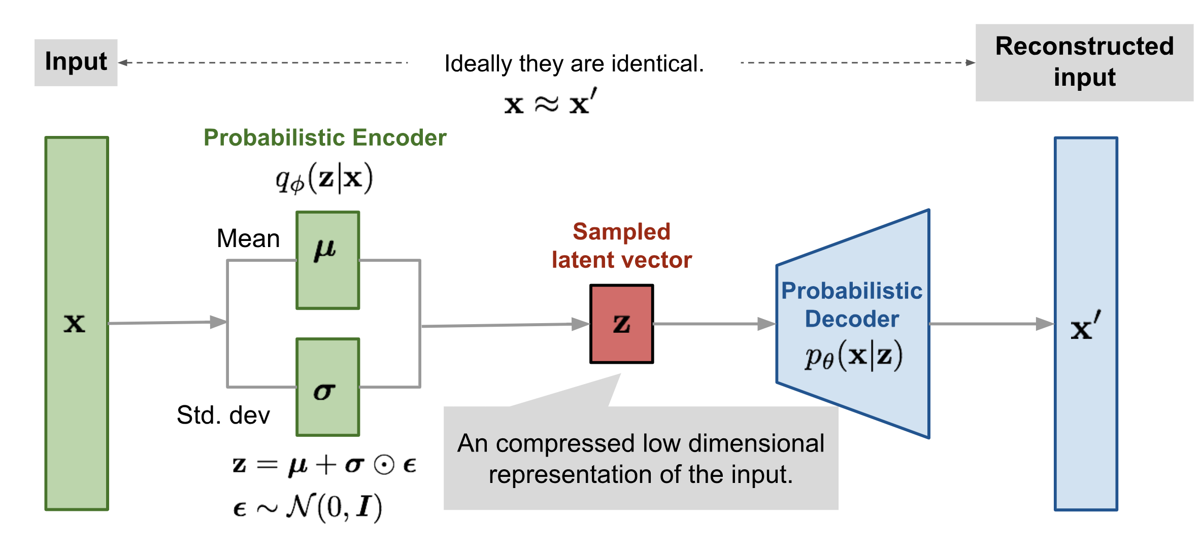
Diagram of a Variational Autoencoder.

Variational Autoencoders are generative models with an encoder-decoder architecture. Just like a standard autoencoder, VAEs are trained in an unsupervised manner where the reconstruction error between the input x and the reconstructed input x’ is minimized. However, in order to introduce some regularization of the latent space, the input is encoded as a distribution over the latent space rather than encoded as a single point.

Generating New Images

To generate a random, new sample that is similar to the training data, you can simply remove the encoder portion of the VAE and randomly sample from the latent distribution. This will give you a latent vector z which can then be decoded using the decoder to produce the new sample x’.

Math Derivation

Now that you have some intuition of how VAEs work, let’s dive into the maths behind VAEs!

Kullback–Leibler Divergence

Let’s first define the Kullback–Leibler (KL) divergence (also called relative entropy). KL divergence is a measure of how one probability distribution is different from a second, reference probability distribution.

For discrete probability distributions P(x) and Q(x) defined on the same probability space, the KL divergence from Q(x) to P(x) is defined as:

The KL divergence has the following properties:

1. 

2. 

The first property will come in handy for later in the derivation and the proof can be found in this post. The second property indicates that KL divergence is not symmetric and therefore, not a distance metric (hence why the term is called a “divergence”).

Variational Inference

VAEs sample values of z that are likely to have produced x. Intuitively, this can be done by sampling from the posterior distribution p(z|x):

However, p(x) is intractable — therefore, making the whole term intractable:

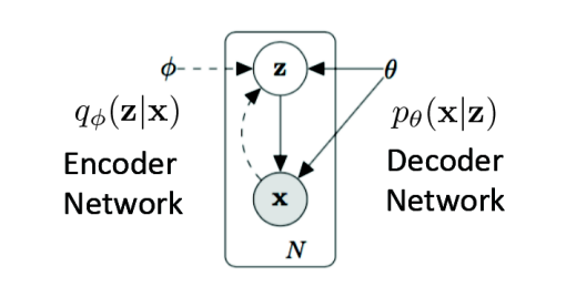
The solution to this issue is to use variational inference to approximate p(z|x) using a tractable distribution q(z|x).

The standard VAE directed graphical model.

Objective Function

We can approximate p(z|x) with q(z|x) by minimizing the KL divergence from q(z|x) to p(z|x):

Let’s manipulate this equation such that we can isolate for p(x) in a single term (you’ll see why later).

Note: all summations are in terms of z.

Substitute p(z|x) using:

Note that:

Therefore,

Rearranging, we get:

Earlier we saw that p(x) is intractable, so how do we maximize the KL-divergence? We use the Evidence Lower Bound (ELBO)!

Evidence Lower Bound

In ELBO, we call the likelihood function evaluated at Θ the evidence.

The intuition behind why this quantity is called the “evidence” is that if we have chosen the right model p and parameters Θ, then we should expect to see a high marginal probability of our observed data p(x; Θ).

ELBO is defined as the lower bound on the evidence:

The derivation of the ELBO is as follows (for now we will drop the Θ in the likelihood function to simplify the math a bit, but assume that it’s there):

Now, we can use Jensen’s inequality since we know that the logarithm function is strictly concave.

Earlier we saw that:

Plugging into Jensen’s inequality, “f” is the logarithm function and “x” is the term p(z, x) / q(z | x):

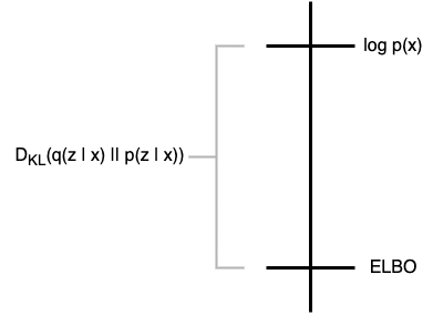
Now, we have solved for ELBO. So then what do we do with this? Notice how the KL divergence is the difference between log(p(x)) and ELBO:

We can visualize this as such:

We know that:

1. ELBO is the lower bound of log(p(x)):

1. KL divergence must be greater or equal to zero:

1. The objective is to minimize the KL divergence by learning the parameters of the variational distribution q and log(p(x)) does not depend on q.

Therefore, we can conclude that by maximizing the ELBO, we are essentially minimizing the KL divergence. You can visualize this by moving the ELBO upwards, closing in on the gap, and decreasing the KL divergence.

Now let’s rewrite the objective function such that it maximizes the ELBO:

Interpretation of ELBO

So let’s try to interpret what the above equation means.

The first term is the expectation of the log-likelihood of observing x given z. Since there is a deterministic function between z and x’, the first term can be rewritten as:

This means that the first term of the ELBO is proportional to the negative squared reconstruction error. Therefore, by maximizing the log-likelihood term, we are essentially minimizing the reconstruction error!

The second term is the negative KL divergence of the variational distribution q(z|x) to the prior p(z). The prior can be chosen and is usually set to be the standard multivariate Gaussian distribution:

The latent vector z can be expressed by sampling from this distribution and transforming it to have mean μ and variance σ:

Due to overfitting, the latent space of an autoencoder can be extremely irregular. For example, close points in latent space can produce very different decoded data. By making the encoder return a distribution over the latent space instead of a single point, regularization is introduced. By maximizing the second term, we are minimizing the KL divergence of the variational distribution to the standard multivariate Gaussian distribution:

This encourages points with the same content to cluster together in the latent space. Therefore, the second term of the ELBO is a regularization term.

Thanks for reading!

Citations

1. https://towardsdatascience.com/understanding-variational-autoencoders-vaes-f70510919f73
2. http://cs229.stanford.edu/notes-spring2019/cs229-notes8-2.pdf
3. https://en.wikipedia.org/wiki/Kullback%E2%80%93Leibler_divergence
4. https://jaan.io/what-is-variational-autoencoder-vae-tutorial/
5. https://pillowlab.wordpress.com/2019/02/10/reductions-in-representation-learning-with-rate-distortion-theory/